A Study of Neural Network Architecture and the Mathematics of Backpropagation

Abstract

Artificial Neural Networks (ANNs) are one of the fundamental building blocks of modern machine learning and deep learning. They have demonstrated remarkable success in a wide range of applications, including image recognition, natural language processing, recommendation systems, healthcare, and financial forecasting. Although inspired by biological neural systems, ANNs are mathematical models designed to learn complex relationships directly from data rather than accurately replicating the functioning of the human brain.

The performance of a neural network depends largely on its ability to learn suitable model parameters from training data. This learning process is driven by optimization algorithms that minimize a predefined loss function. Among these, backpropagation combined with gradient-based optimization has become the standard approach for training neural networks since past few years.

This paper introduces the basic architecture of artificial neural networks, explains how information propagates through the network during inference, and develops the mathematical foundations of the backpropagation algorithm. The objective is to provide an intuitive as well as mathematical understanding of how neural networks learn from data.

1. Introduction

Artificial Neural Networks (ANNs) are computational models that learn patterns directly from data. Unlike traditional rule-based algorithms, neural networks improve their performance by adjusting internal parameters through a training process, allowing them to model highly complex and non-linear relationships.

Today, neural networks form the foundation of many state-of-the-art machine learning systems. They are used in applications such as computer vision, speech recognition, machine translation, recommendation systems, fraud detection, autonomous driving, and scientific research. Their ability to learn hierarchical representations from large datasets has made them one of the most widely used techniques in artificial intelligence.

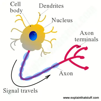
The term neural network originates from the fact that these models were loosely inspired by the organization of neurons in the human brain. However, modern artificial neural networks are mathematical abstractions rather than biologically accurate simulations. Their strength lies not in mimicking the brain, but in efficiently learning parameterized functions that map inputs to desired outputs. We are just modelling a real world situation into a mathematical model using the data available to us.

This paper focuses on two fundamental concepts underlying neural networks:

1. Forward propagation, which computes the network's prediction for a given input.

2. Back propagation, which efficiently computes the gradients required to update the network parameters during training.

Before discussing these algorithms, we first examine the structure of an artificial neural network and the role of its individual components.

2. Structure of a Neural Network

The human brain consists of billions of interconnected neurons that communicate through electrical and chemical signals. Although artificial neural networks were originally inspired by this biological concept, they are not intended to replicate the biological processes of the brain. Instead, they provide a mathematical framework for learning complex relationships from data.

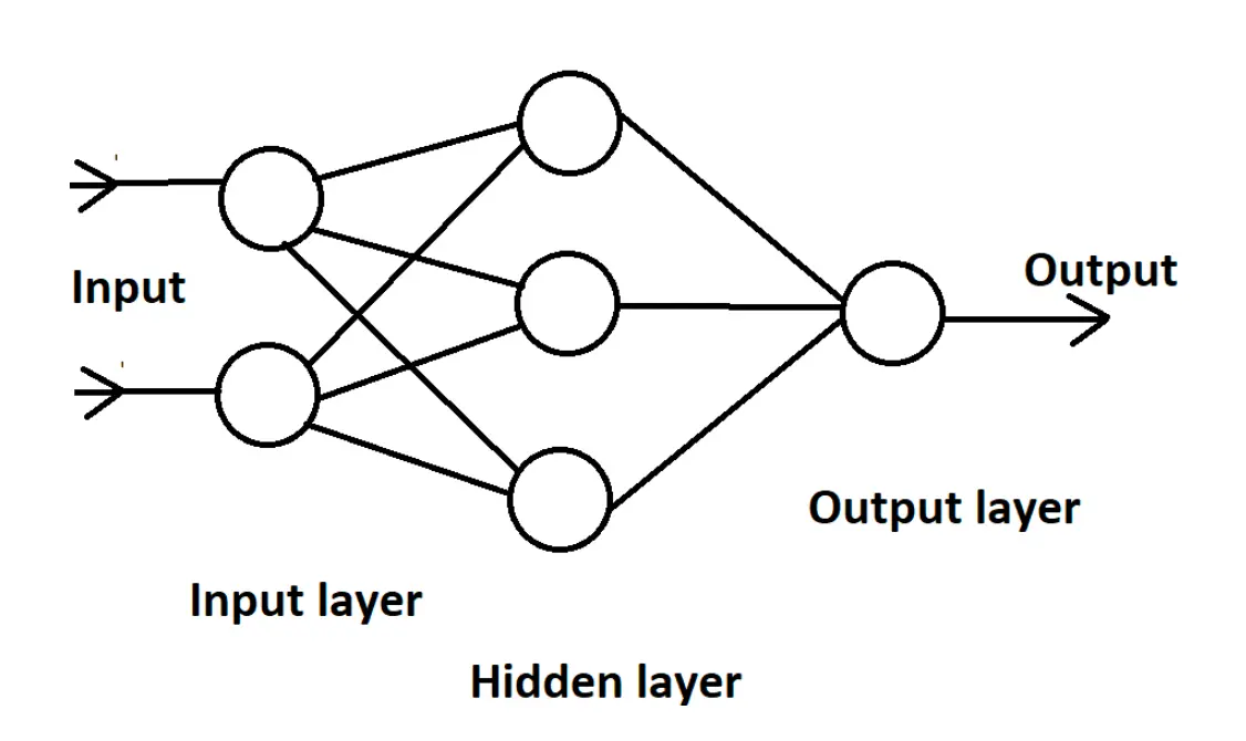
An artificial neural network (ANN) is composed of simple computational units called neurons (or nodes) that are organized into layers. Each neuron receives one or more inputs, performs a mathematical computation, applies an activation function, and produces an output that is passed to neurons in the next layer.

A feedforward neural network typically consists of three types of layers:

• Input Layer: Receives the input features and passes them to the network. No computation is performed at this layer apart from forwarding the input values.

• Hidden Layer(s): Perform intermediate computations that enable the network to learn increasingly complex representations of the input data. A network may contain one or many hidden layers.

• Output Layer: Produces the final prediction. The number of output neurons depends on the learning task. For example, binary classification typically uses a single output neuron, whereas multi-class classification uses one output neuron for each class.

Each neuron in one layer is connected to neurons in the next layer through weights, which determine the strength of the connections. In addition, every neuron is associated with a bias, which allows the model to shift the activation independently of the inputs. During training, the network learns appropriate values for these weights and biases so that its predictions become increasingly accurate.

The overall architecture of a neural network is illustrated in this figure below.

The complexity of a neural network depends primarily on:

• the number of hidden layers (network depth),

• the number of neurons in each layer (network width), and

• the pattern of connections between neurons.

While the examples presented in this paper use relatively small networks to simplify the mathematical derivations, the same underlying principles extend naturally to much larger neural networks used in modern deep learning systems.

3. Operation of a Neural Network

The primary objective of a neural network is to learn a function that maps a given input to the desired output. During inference (or prediction), information flows from the input layer through one or more hidden layers until it reaches the output layer. This one-way flow of information is known as forward propagation (or feed forward propagation).

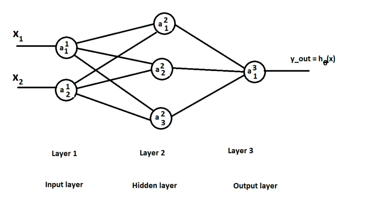
To illustrate the underlying mathematics, consider a feedforward neural network consisting of:

• an input layer with two neurons,

• one hidden layer with three neurons, and

• an output layer with one neuron.

Although modern neural networks often contain many more layers and neurons, the same principles apply regardless of the network's size.

Let the activation of the neuron in the layer be denoted by where:

• the superscript (i) denotes the layer number, and

• the subscript (j) denotes the neuron within that layer.

For the input layer, the activation values are simply the input features themselves. For every subsequent layer, the activation values are computed using the outputs from the previous layer, together with the network's learned parameters (weights and biases).

Thus, every neuron performs two operations:

1. Compute a weighted sum of its inputs together with a bias.

2. Apply an activation function to introduce non-linearity.

These two steps are repeated layer by layer until the network produces its final prediction.

The mathematical details of this computation are presented in the next section.

3.1 Forward Propagation

Forward propagation is the process of computing the output of a neural network for a given input. At each layer, every neuron receives the activations from the previous layer, computes a weighted sum, adds a bias term, and then applies an activation function.

For a neuron in layer (l), the weighted input is given by

where:

• is the weight matrix connecting layer (l-1) to layer (l),

• is the bias vector for layer (l),

• is the activation vector from the previous layer, and

• is commonly referred to as the pre-activation or weighted input.

The activation values for the current layer are then computed by applying an activation function:

where denotes the activation function.

Sigmoid Activation Function

For simplicity, this paper uses the sigmoid activation function:

The sigmoid function maps any real-valued input to the interval , making it suitable for demonstrating the mathematical concepts presented in this paper.

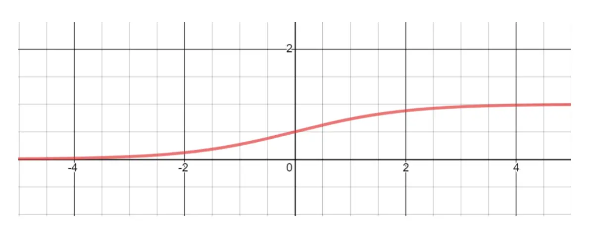
Although sigmoid is no longer the default choice for hidden layers in modern deep learning—where activation functions such as ReLU and its variants are generally preferred—it remains one of the simplest activation functions for understanding forward propagation and backpropagation because its derivative has a convenient analytical form.

Once the activations of one layer have been computed, they become the inputs to the next layer. This process continues sequentially until the output layer is reached. The final activation of the output layer represents the network's prediction.

The parameters (W) and (b) are initially assigned random values. During training, these parameters are iteratively updated so that the network's predictions become increasingly close to the expected outputs. The algorithm responsible for learning these parameters is discussed in the following sections.

3.2 Examples of Forward Propagation

The mathematical equations introduced in the previous section can be better understood through a few simple examples. For these examples, assume that the neural network has already been trained and that the values of the weights and biases are known. Our objective is simply to compute the network's prediction using forward propagation.

Example 1: Single-Layer Neural Network

Consider a neural network consisting of:

• an input layer with two neurons, and

• an output layer with one neuron.

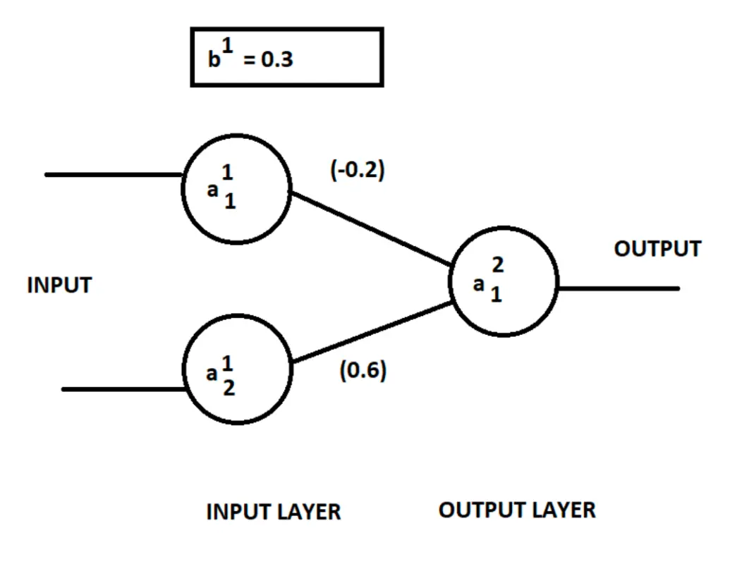
The learned parameters are also shown in the above figure.

Suppose the network receives the following input:

Using the forward propagation equations,

Applying the sigmoid activation function,

Now consider a second input:

The weighted input becomes

and therefore,

If a classification threshold of 0.5 is chosen, the first input would be classified as Class 0, while the second would be classified as Class 1.

This example demonstrates how different inputs produce different activation values even though the network parameters remain unchanged.

Example 2: Neural Network with One Hidden Layer

Now consider a slightly deeper neural network consisting of:

• an input layer,

• one hidden layer with two neurons, and

• an output layer with one neuron.

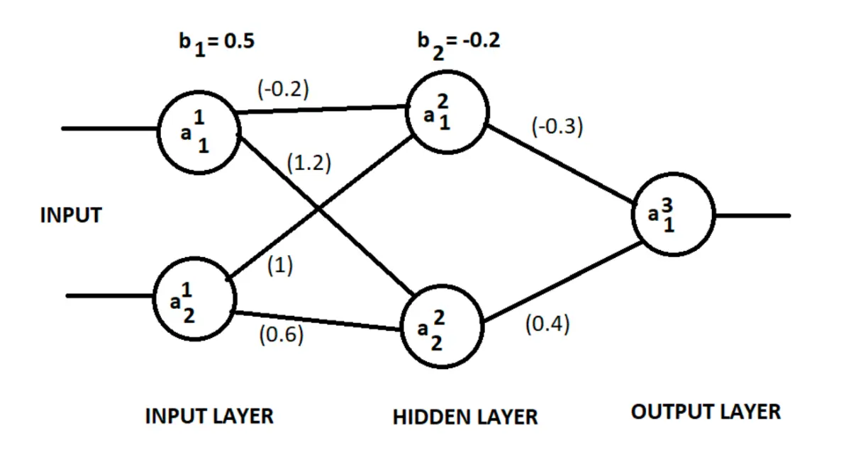For the input

the hidden-layer activations are

The output neuron then computes

If the classification threshold is chosen as 0.6, this input is classified as Class 0.

This example illustrates an important characteristic of neural networks: each hidden layer transforms the input into a new representation before passing it to the next layer. As networks become deeper, they can learn increasingly complex representations, enabling them to solve problems that cannot be modeled using a single linear transformation.

3.3 Why Do We Need Backpropagation?

In the previous sections, we assumed that the values of the network's weights and biases were already known. In practice, however, these parameters are not known beforehand—they must be learned from data. That's where the machine learns (and machine learning comes into picture)

A neural network typically begins with randomly initialized weights and biases. As a result, its initial predictions are usually far from the desired outputs. The objective of training is therefore to iteratively adjust these parameters so that the network's predictions become increasingly accurate.

To measure how well the network performs, we define a loss function (also called a cost function). The loss function quantifies the difference between the network's predictions and the true labels. A smaller loss indicates better performance, while a larger loss indicates that the model's predictions are less accurate.

Training a neural network is therefore an optimization problem: we seek the values of the weights and biases that minimize the loss function.

The most widely used optimization algorithm for this purpose is gradient descent. At every iteration, gradient descent updates each parameter in the direction that most rapidly decreases the loss. The update rules are

where

• (J) is the loss function,

• () is the learning rate, and

• () and () are the gradients of the loss with respect to the model parameters.

The learning rate determines the size of each update step. Choosing an appropriate learning rate is important: a value that is too small results in slow training, whereas a value that is too large may prevent the optimization algorithm from converging.

The remaining question is:

How do we efficiently compute the gradients of the loss function with respect to every weight and bias in the network?

For a neural network containing thousands or even millions of parameters, computing these gradients manually would be infeasible.

This is precisely the purpose of the backpropagation algorithm. Backpropagation efficiently computes the gradients of the loss function with respect to every trainable parameter by repeatedly applying the chain rule of calculus. These gradients are then used by gradient descent (or one of its variants) to update the network parameters.

Loss Function

For consistency with the remainder of this paper, we use the Mean Squared Error (MSE) loss for a dataset containing (m) training examples:

where

• () is the prediction for the () training example,

• () is the corresponding ground-truth value, and

• (m) is the number of training examples.

Although modern neural networks often use different loss functions—for example, binary cross-entropy for binary classification and categorical cross-entropy for multi-class classification—mean squared error is mathematically simpler and is therefore sufficient for illustrating the principles of backpropagation developed in this paper. The choice of the loss function depends on the problem we are trying to solve.

Having defined both the optimization objective and the parameter update rules, we are now ready to derive the gradients required for training the network.

3.4 Back propagation

The objective of training a neural network is to find the values of the weights and biases that minimize the loss function. As discussed in the previous section, gradient descent requires the gradient of the loss with respect to every trainable parameter.

The challenge is that each parameter influences the final prediction indirectly through several intermediate computations. Consequently, the loss does not depend on a weight or bias directly; instead, the dependency passes through a sequence of mathematical operations performed during forward propagation.

Backpropagation provides an efficient solution to this problem. Rather than computing each gradient independently, it applies the chain rule of calculus to propagate the error from the output layer backward through the network, computing the required gradients for every parameter.

The algorithm consists of four conceptual steps:

1. Perform forward propagation to compute the network's prediction.

2. Evaluate the loss by comparing the prediction with the expected output.

3. Propagate the error backward through the network using the chain rule.

4. Update the weights and biases using gradient descent.

These steps are repeated for many training iterations until the loss converges or another stopping criterion is satisfied.

To understand the mathematics, we first consider the simplest possible neural network consisting of one input neuron connected to one output neuron.

Example: Single-Layer Neural Network

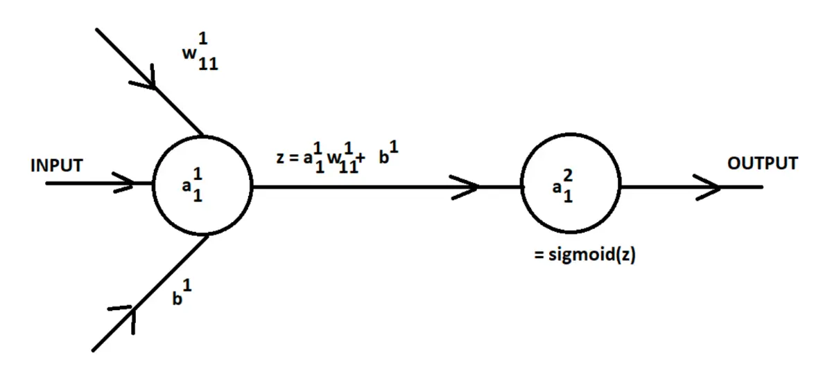
Assume the network shown above figure, where

and the loss for a single training example is

where

• (x) is the input,

• (w) is the weight,

• (b) is the bias,

• (a) is the predicted output, and

• (y) is the target value.

Our goal is to compute

and

which are required by gradient descent.

Applying the Chain Rule

Notice that the loss is not expressed directly as a function of the weight. Instead, the dependency follows the sequence

Therefore, the chain rule gives

Each term can be computed independently.

Since

we obtain

The derivative of the sigmoid activation function is

Therefore,

Finally,

Combining these results,

which gives the gradient of the loss with respect to the weight.

Similarly,

Since

we obtain

These two expressions provide the gradients required to update the weight and bias using gradient descent.

Extending to Deeper Networks

The derivation above considers only a single-layer network, but the same principle applies to networks with multiple hidden layers.

The only difference is that the dependency between a parameter and the loss now passes through many intermediate variables. Consequently, the chain rule contains additional terms corresponding to each layer of the network.

For example, in a three-layer network, the dependency becomes

[ J]

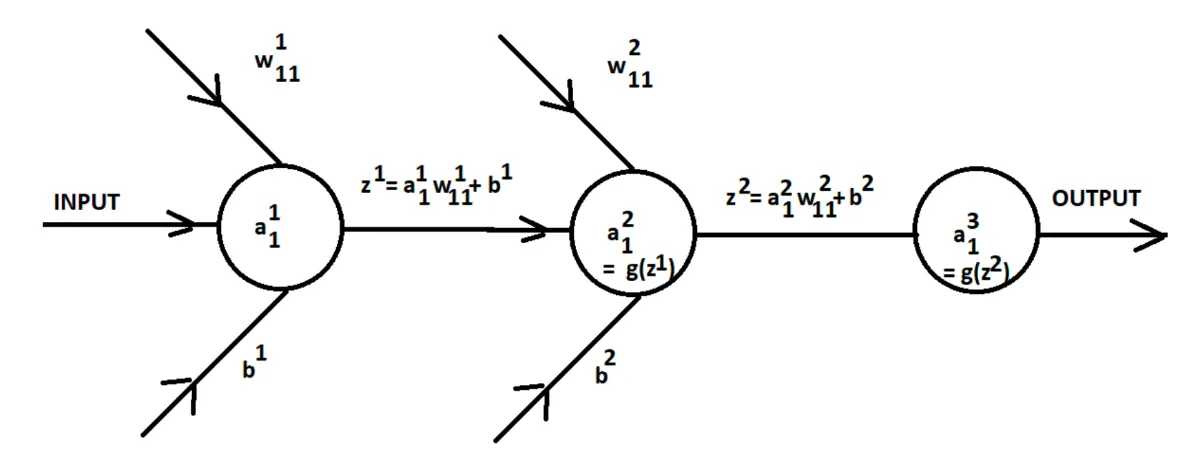
The gradient is obtained by multiplying the derivatives along this computational path.

Although the mathematical expressions become longer, the underlying idea remains unchanged: backpropagation repeatedly applies the chain rule to compute the gradient of the loss with respect to every trainable parameter.

In practice, these computations are implemented using vectorized matrix operations, allowing modern deep learning frameworks to efficiently train networks containing millions or even billions of parameters.

4. Additional Notes

The previous sections described the mathematical foundations of forward propagation and backpropagation. Before concluding, a few practical aspects of training neural networks are worth discussing.

Learning Rate

The learning rate () controls the magnitude of each parameter update during optimization. Selecting an appropriate learning rate is critical for successful training.

• A learning rate that is too small results in slow convergence.

• A learning rate that is too large may cause the optimization process to overshoot the optimum or fail to converge.

In practice, the learning rate is treated as a hyperparameter and is selected through experimentation or automated hyperparameter tuning techniques.

Network Architecture

The performance of a neural network depends heavily on its architecture, including the number of hidden layers, the number of neurons in each layer, and the choice of activation functions.

There is no universally optimal architecture. The appropriate design depends on the complexity of the problem, the amount of available training data, computational resources, and the desired trade-off between accuracy and efficiency.

Activation Functions

Although this article uses the sigmoid activation function for mathematical simplicity, modern neural networks frequently employ activation functions such as ReLU, Leaky ReLU, GELU, and SiLU, particularly in hidden layers. These functions generally improve optimization and help mitigate issues such as vanishing gradients.

Optimization Algorithms

While this article focuses on gradient descent, modern deep learning commonly employs variants such as Stochastic Gradient Descent (SGD) with momentum, Adam, AdamW, and RMSProp. These algorithms often achieve faster convergence and improved training stability.

Mini-batch Training

Instead of computing gradients using the entire training dataset (batch gradient descent) or a single training example (stochastic gradient descent), modern neural networks are typically trained using mini-batches.

Mini-batch gradient descent provides a practical balance between computational efficiency and convergence stability, making it the standard approach in contemporary deep learning frameworks.

Automatic Differentiation

Although this article derives the gradients manually to explain the underlying mathematics, modern deep learning libraries such as PyTorch, TensorFlow, and JAX compute these gradients automatically using automatic differentiation. Nevertheless, understanding the mathematical principles behind backpropagation remains essential for designing, debugging, and improving neural network models.

5. Conclusion

This article introduced the fundamental concepts underlying artificial neural networks and explained the mathematical principles that enable them to learn from data.

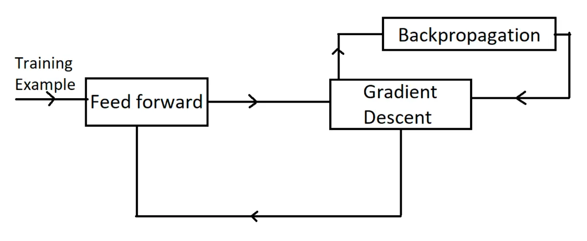
We first examined the architecture of a feedforward neural network and the process of forward propagation, in which information flows through successive layers to produce a prediction. We then formulated the training problem as an optimization task, where the objective is to minimize a loss function by adjusting the network's weights and biases.

The central focus of the article was the backpropagation algorithm. By employing the chain rule of calculus, backpropagation efficiently computes the gradient of the loss function with respect to every trainable parameter in the network. These gradients are subsequently used by optimization algorithms such as gradient descent to iteratively improve the model's performance.

Although modern deep learning models are significantly larger and more sophisticated than the examples presented here, the underlying mathematical principles remain the same. The concepts of forward propagation, loss computation, gradient calculation, and parameter updates continue to form the foundation of virtually all supervised deep learning algorithms.

A thorough understanding of these principles provides the basis for studying more advanced neural network architectures and optimization techniques used in contemporary machine learning research and applications.

Note

This article was originally published as a paper by the author on researchgate. This article is a simplified re-write of the paper generated with the help of AI tools.